Analysing quantity responses
Quantity Response questions are used to collect open-ended numeric responses in a survey. This type of data would usually be values such as amounts of money, volumes, areas etc. Quantity Response data can be analysed as follows:
- A list of Quantity Responses can be produced either for all respondents or for respondents selected on the basis of a filter specification. This is done in the same way as a list of Literal Responses
- Statistics of the quantity values can be calculated either for all respondents or for respondents selected on the basis of a filter specification.
A Derived Variable can be set up to allocate the quantity data into coded ranges. These are used as an analysis or break variable on a table.
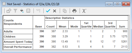
Overview of descriptive statistics
You can produce a table of descriptive statistics which shows, for each variable in the specification, the mean, mode, median, quartiles, sum, min, max, range, standard deviation, and variance, standard error of the mean, skewness and kurtosis. Any of the statistics can be excluded using the Descriptive Statistics tab on the Analysis Definition dialog.
Descriptive statistics can be calculated for all cases or for those selected on the basis of a Filter Specification. Missing values such as No Reply will be excluded from statistical calculations. The statistics can also be weighted, perhaps to correct some imbalance in the sampling, by providing a suitable weight specification.
To describe each of the statistics that may be calculated assume that a survey of households was conducted. As part of that survey the number of persons living in the household was requested. The following replies were received from the eleven households interviewed:
1, 2, 3, 4, No Reply, 3, 4, 5, 4, 6, 2
Statistic | Description |
Mean | This is often called the average, and is defined as the sum of the items divided by the number of items. Mean = (1 + 2 + 3 + 4 + 3 + 4 + 5 + 4 + 6 + 2) = 34 10 = 3.4 Since one respondent gave no reply, the mean and all other statistics are calculated using a sample of 10. |
Mode | The mode of a distribution is the most frequent or most popular item. If two values tie for the mode, Snap will choose the lower. Mode = 4, since 4 is the most frequently occurring value (three occurrences). |
Quartile 1 | 25% through a range of values |
Median | The midpoint or 50% through a range of values. To calculate the median, the items of the distribution are arranged in order of magnitude starting with either the smallest or the largest, then: if the number of items is odd, the median is the value of the middle item. if the number of items is even, the median is the mean of the two middle items. 1, 2, 2, 3, 3, 4, 4, 4, 5, 6 Median = (3 + 4) ÷ 2 = 3.5 |
Quartile 3 | 75% through a range of values. |
Sum | The sum is calculated by adding all the values of a distribution. Sum = 1 + 2 + 3 + 4 + 3 + 4 + 5 + 4 + 6 + 2 = 34 |
Minimum | The minimum is the smallest value of the distribution. Minimum = 1 |
Maximum | The maximum is the largest value of the distribution. Maximum = 6 |
Range | The range shows the spread of the distribution and is calculated by subtracting the smallest value (minimum) from the largest value (maximum). Range = 6 – 1 = 5 |
Standard Deviation | The standard deviation is a measure of dispersion of values in a distribution. It gives an indication of how much the values deviate from the mean. Thus, a distribution with a large range would have a larger standard deviation than one with a small range. The standard deviation is calculated as: 
where xi is each value in the distribution,
Standard Deviation = 1.428286 |
Variance | The variance is another measure of dispersion of values in a distribution and is calculated as the square of the standard deviation: Variance = 2.04 Snap calculates the standard deviation and variance by assuming the data represents a sample rather than an entire population. |
Standard Error of the Mean | The standard error of the mean is calculated by dividing the standard deviation by the square root of the number of items in the sample. It is defined as the standard deviation of the distribution of the sample mean and gives an indication of how far individual scores deviate from the mean score shown. The larger the sample, and/or the closer the individual scores are to the mean score, the smaller the standard error. Standard Error of the Mean = 1.428286 10 = 0.451664 |
Skewness | A distribution that is not symmetrical but has more cases toward one end of the distribution than the other is called skewed. The measures of central tendency (mean, mode and median) can vary considerably. If the mean is larger than the mid point of the range (the median) and the most frequently occurring value (the mode), the sample is said to be positively skewed. If the mean is smaller than the mid point of the range (the median) and the most frequently occurring value (the mode), the sample is said to be negatively skewed. A small skewness value (close to 0) indicates that the data is evenly distributed about the mean. With this type of distribution it would be expected that the values for mean, mode and median be similar. The skewness of the example is 0.098843 indicating a small positive skewness. |
Kurtosis | Kurtosis also gives an indication of the shape of a distribution in the form of the extent to which, for a given standard deviation, the data clusters around a central point. A positive value for kurtosis indicates a distribution that is more peaked than usual. A distribution of this type would typically have most of the values clustered around a central point. A negative value for kurtosis indicates a flatter or more widely dispersed distribution. The kurtosis for the example is -0.75202 |